Understanding Autograd and Neural Network in PyTorch

Lars Davidson
Division of Fluid Dynamics
Dept. of Mechanical Engineering
Chalmers University of Technology
SE-412 96 Gothenburg, Sweden
lada@chalmers.se

from datetime import datetime
print(datetime.today().strftime('%Y-%m-%d'))

2026-07-17

Introduction

At Wikipedia, Neural network (NN) is described as a computational model inspired by the structure and functions of biological neural networks. Artificial neuron models that mimic biological neurons have also recently been investigated and shown to significantly improve performance. These are connected by edges, which model the synapses in the brain. Each artificial neuron receives signals from connected neurons, which processes them and sends a signal to other connected neurons. The "signal" is a real number, and the output of each neuron is in this report computed by a linear function of its inputs which is multiplied by an activation function. The strength of the signal at each connection is determined by the weights and biases of the linear function, which are updated during the learning process in order to reduce the loss. The loss is defined as the difference between the predicted output and the correct solution (called the target).

Tensors

Tensor in the computer world simply means a multidimensional array. A scalar is a zero-dimensional tensor, which is a single number. A leaf tensor is a tensor that is a leaf (in the sense of a graph theory) of a computation graph. I will discuss leafs below.

The requires_grad = True for a tensor tells PyTorch that it should remember how this tensor is used in further computations. For now, think of tensors with requires_grad=True as variables, while tensors with requires_grad=False as constants.

Leafs and requires_grad

Let’s start by creating a few tensors and checking their properties requires_grad and is_leaf.

import torch
a = torch.tensor([3.], requires_grad=True)
b = a * a

c = torch.tensor([5.])
d = c * c

print(a.requires_grad)
print(b.requires_grad)
print(c.requires_grad)
print(d.requires_grad,'\n')
print(a.is_leaf)
print(b.is_leaf)
print(c.is_leaf)
print(d.is_leaf)

True
True
False
False 

True
False
True
True

The a = torch.tensor([3.], requires_grad=True) statement tells PyTorch to

1. store all mathematical operations (addition, multiplication ...) involving $a$
2. store the gradient of any new tensor that is created from $a$

In PyTorch, leaf tensors are either

1. direct input (i.e. not calculated from other tensors) and have requires_grad=True. Example: neural network weights that are randomly initialized.
2. do not require gradients at all, regardless of whether they are direct input or computed. These are just constants.

Hence, $a$ is a leaf because it is an input variable, and $b$ is not because it is a result of a multiplication. $a$ is set to requires_grad, so $b$ inherits this property.

$c$ is a leaf because it is an input variable

The reason d.is_leaf is True stems from the PyTorch convention that all tensors for which requires_grad is set to False are considered leaf tensors.

All Tensors that have requires_grad = False will be leaf tensors by convention. Mathematically, $d$ is not a leaf (since it results from another operation, $c * c$), but gradient computation will never extend beyond it. In other words, there will not be any derivative with respect to $c$. This allows $d$ to be treated as a leaf.

The requires_grad property is inherited, i.e. $d$ has requires_grad = False which is inherited from $c$.

a = torch.tensor([7.], requires_grad=True)
b = torch.tensor([8.], requires_grad=True)

The grad_fn attribute

I create another tensor $Q$ from $a$ and $b$ as \begin{eqnarray} Q=a^3 - 4b \end{eqnarray}

Q = a**3 - 3*b

In PyTorch, tensors can have a grad_fn attribute. When a tensor is created by a mathematical operation, PyTorch keeps track of the operation that created it using the grad_fn. This is part of the computational graph, which is a directed acyclic graph (DAG).

print(a.requires_grad)
print(b.requires_grad)
print(Q.requires_grad)
print(a.grad)
print(b.grad)
print(Q.grad_fn)

True
True
True
None
None
<SubBackward0 object at 0x7f9cfbafd120>

$a$ and $b$ are created with requires_grad=True and that attribute is inherited by $Q$. The tensors a.grad and b.grad are still not defined because I have not executed the .backward() command.

The grad_fn is an object that represents the operation that created the tensor. It has a backward method, which is used to compute the gradients during the backward pass. If a tensor is created by the user directly (e.g., torch.tensor(2.0, requires_grad=True)), its grad_fn is None because it is a leaf tensor in the computational graph.

Now I will compute the gradients by a backward pass. Verify that the gradients $\partial Q/\partial a$ and $\partial Q/\partial b$ have been computed

Q.backward()
print('dQ/da',a.grad)
print('dQ/db',b.grad)

dQ/da tensor([147.])
dQ/db tensor([-3.])

The .grad_fn attribute is used to analyze the mathematical operations for $Q$. Below I visualize the autograd graph using the agtree2dot package which can be downloaded at https://fleuret.org/francois/

Autograd graph

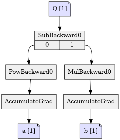
The figure above was generated by the code in the cell below.

import agtree2dot
agtree2dot.save_dot(Q,
   {
    a: 'a',
    b: 'b',
    Q: 'Q',
   },
   open('./Q.dot', 'w'))
# dot -T png Q.dot -o Q.png 

print(Q.grad_fn)
print(Q.grad_fn.next_functions)

<SubBackward0 object at 0x7f9cfbafd270>
((<PowBackward0 object at 0x7f9c162d6b60>, 0), (<MulBackward0 object at 0x7f9c162d4160>, 0))

The first line (object = SubBackward0) of the output shows that $Q$ is obtained by a subtraction i.e. $-3b$. This corresponds to the second box from the top in the graph above

The second line shows the two prior operations (object = PowBackward0 and MulBackward0) which correspond to $a^3$ and the multiplication of $3$ and $b$. They form two branches, $0$ and $1$. Branch 0 is shown below

print(Q.grad_fn.next_functions[0][0].next_functions)
print(Q.grad_fn.next_functions[0][0].next_functions[0][0].\
      variable)
print(Q.grad_fn.next_functions[0][0].next_functions[0][0].\
      variable is a)

((<AccumulateGrad object at 0x7f9cfbafd420>, 0),)
tensor([7.], requires_grad=True)
True

Line 1 shows that the variable is accumulated. The value of the variable is printed at the second line and the third line confirms that it is $a$. Hence, you see that branch 0 is the left branch in the graph above. Next, let's look at branch 1.

print(Q.grad_fn.next_functions[1][0])
print(Q.grad_fn.next_functions[1][0].next_functions)
print(Q.grad_fn.next_functions[1][0].next_functions[0][0].\
      variable)
print(Q.grad_fn.next_functions[1][0].next_functions[0][0].\
      variable is b)

<MulBackward0 object at 0x7f9c162d7bb0>
((<AccumulateGrad object at 0x7f9c162d4700>, 0), (None, 0))
tensor([8.], requires_grad=True)
True

The first line says that it is a multiplication (of $3$ and $b$). On the second line you see that the variable has been accumulated. The value of the variable is printed at line 3 and line 4 confirms that the variable is indeed $b$. Branch 1 corresponds to the right branch in the graph above.

Let's introduce another variable, $P$

\begin{eqnarray} Q=a^3 - 3b, \quad P = Q^2 \quad \Rightarrow \quad P=a^6 -6a^3b + 9b^2 \end{eqnarray}

In Python it reads

a = torch.tensor([2.], requires_grad=True)
b = torch.tensor([8.], requires_grad=True)
Q = a**3 - 3*b
P = Q**2 

The gradient of $P$ with respect to $a$ and $b$ is

\begin{eqnarray*} \partial P/\partial a = \frac{\partial P}{\partial Q} \frac{\partial Q}{\partial a} = 6a^5 - 18a^2b = -384, \quad \partial P/\partial b = \frac{\partial P}{\partial Q} \frac{\partial Q}{\partial b}\\ = -6a^3 + 18b = 96 \end{eqnarray*}

Note that Pytorch uses the chain-rule when computing the gradients above.

Verify that the Pytorch command backward() gives the correct answer.

P.backward()
print('dP/da =',a.grad)
print('dP/db =',b.grad)

dP/da = tensor([-384.])
dP/db = tensor([96.])

Note that the command P.backward() deletes all intermediate gradients. If you want the keep $\frac{\partial P}{\partial Q} = 2Q = 2a^3 - 6b = -32$ you must use the command .retain_grad() command, i.e.

Q = a**3 - 3*b
P = Q**2 
Q.retain_grad()
# in order to avoid accumulation when  P.backward() is called for a second time
a.grad = None
b.grad = None
P.backward()
print('dP/dQ =',Q.grad)
print('dP/da =',a.grad)
print('dP/db =',b.grad)

dP/dQ = tensor([-32.])
dP/da = tensor([-384.])
dP/db = tensor([96.])

Solve the equation $P=a^6 -6a^3b + 9b^2 = 0$ using autograd

Let's solve the equation $P=0$ using autograd.

a = torch.tensor([2.], requires_grad=True)
b = torch.tensor([8.], requires_grad=True)
Q = a**3 - 3*b
P = Q**2 
# Define the variables which should be solved for 
list_parameters = [a,b]

#under-relaxation
alpha = 0.02 

# choose optimizer
optimizer = torch.optim.Adam(params=list_parameters, lr=alpha)

# max number of iterations
max_iter = 200

for n in range(max_iter):

# set a.grad and b.grad to zero
   optimizer.zero_grad() 
# compute dP/da and dP/db (backward step)
   P.backward() 
# update a and b with gradient descent:
# a = a - dP/da*alpha, b = b - dP/db*alpha, 
   optimizer.step() 
# compute new Q (forward step)
   Q = a**3 - 3*b  
# compute new P (forward step)
   P = Q**2

   if n%50 == 0:
      print(f'iteration no: {n}, P: {P.item():.2e}, \
            a: {a.item():.2e}, b: {b.item():.2e}')

iteration no: 0, P: 2.46e+02,             a: 2.02e+00, b: 7.98e+00
iteration no: 50, P: 4.84e-01,             a: 2.82e+00, b: 7.25e+00
iteration no: 100, P: 1.68e-02,             a: 2.79e+00, b: 7.27e+00
iteration no: 150, P: 1.11e-04,             a: 2.79e+00, b: 7.26e+00

autograd finds the solution $a=2.79$ and $b=7.26$ which gives $P\le 1.2 \cdot 10^{-4}$.

Find the coefficients of a polynomial satisfying y = sin(x)

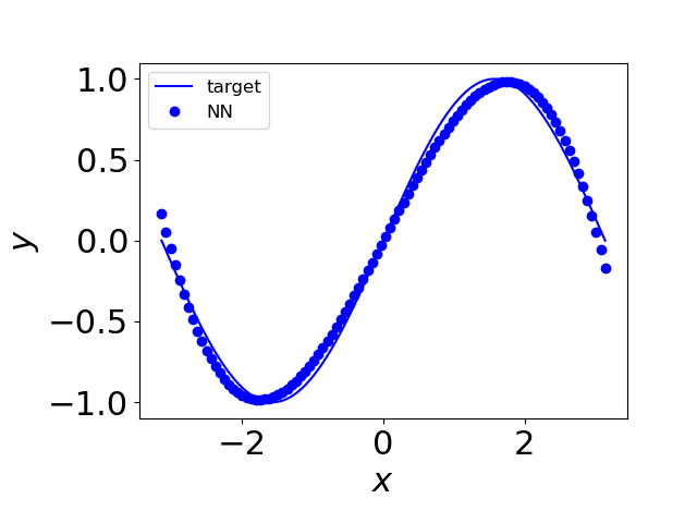
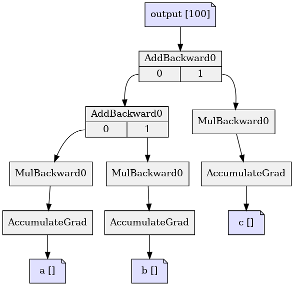
Consider the polynomial $y(x) = a x + b x ^ 2 + c x ^ 3$. I will use autograd to find the coefficients $a$, $b$ and $c$ that satisfies $y = \sin(x)$. The $x$ vector is set to $100$ equidistant points from $-\pi$ to $\pi$, and the coefficients are initialized to zero. Note that the coefficients must be defined by requires_grad=True since they will be updated by autograd.

import torch
import math
import matplotlib.pyplot as plt
x = torch.linspace(-math.pi, math.pi, 100)
y = torch.sin(x)

a = torch.tensor(0.,requires_grad=True)
b = torch.tensor(0.,requires_grad=True)
c = torch.tensor(0.,requires_grad=True)

I create a loop as in the cell above

alpha = 1e-5
max_iter = 4000
for n in range(max_iter):
# compute new y (forward step)
    y_pred = a * x + b * x ** 2 + c * x ** 3 
# compute loss
    L = (y_pred - y).pow(2).sum() 
# retain a, b and c. This is necessary since the backward 
# command would otherwise delete a.grad, b.grad and c.grad 
    a.retain_grad() 
    b.retain_grad() 
    c.retain_grad()  
# compute dL/da, dL/db, dL/dc 
    L.backward() 
    if n % 1000 == 0:
        print(f"\nEpoch {n+1}, L: {L.item():.2e}, \
        a.grad: {a.grad:.2e},  b.grad: {b.grad:.2e},  \
        c.grad: {c.grad:.2e}")
    # update weights using gradient descent.
    a = a - alpha * a.grad
    b = b - alpha * b.grad
    c = c - alpha * c.grad
    # Set the the gradients after updating weights
    a.grad = None
    b.grad = None
    c.grad = None
    
print(f'\na = {a.item():.2e}, b = {b.item():.2e}, \
        c = {c.item():.2e}')

Epoch 1, L: 4.95e+01,         a.grad: -1.98e+02,  b.grad: 2.38e-07,          c.grad: -7.66e+02

Epoch 1001, L: 5.18e+00,         a.grad: -3.12e+01,  b.grad: 0.00e+00,          c.grad: 4.35e+00

Epoch 2001, L: 1.05e+00,         a.grad: -1.09e+01,  b.grad: 0.00e+00,          c.grad: 1.52e+00

Epoch 3001, L: 5.45e-01,         a.grad: -3.79e+00,  b.grad: -2.38e-07,          c.grad: 5.29e-01

a = 8.40e-01, b = 3.53e-10,         c = -9.05e-02

The figure below shows predicted $y$ v. $x$

$y$ v. $x$

The autograd graph is seen below.

Autograd graph for computing $a$, $b$ and $c$

Predict the sinus curve with Neural Network (NN)

I will predict the sinus curve with NN. The code is given below.

import torch
import math
import sys
import matplotlib.pyplot as plt
from torch import nn
import agtree2dot

x = torch.linspace(-math.pi, math.pi, 20) # create x 
y = torch.sin(x)

X = x.view(-1,1)    #makes the shape X[N,1]
Y = y.view(-1,1)

# Build the model:
class NN_sinus(nn.Module):
    def __init__(self):
        super().__init__()
# axis 0: number of inputs
        self.input   = nn.Linear(1, 10) 
        self.hidden1 = nn.Linear(10, 10)
# axis 1: number of outputs
        self.hidden2 = nn.Linear(10, 1) 

    def forward(self, a0):
        a1 = nn.functional.relu(self.input(a0))
        a2 = nn.functional.relu(self.hidden1(a1))
        a3 = self.hidden2(a2) #output

        return a3

# Create the model
# the same initial weights and seed are created every time
torch.manual_seed(42) 
model = NN_sinus()

# Define the loss function and the optimizer
loss_fn = nn.MSELoss()
# learning_rate = 0.0001
learning_rate = 0.001
# choose optimizer
optimizer = torch.optim.Adam(params = model.parameters(), \
                             lr = learning_rate)

max_iter = 1000
for n in range(max_iter):
# predict new y (forward step)
  y_pred = model(X) 
# compute the loss, L,  i.e. difference between 
# target and prediction
  L = loss_fn(y_pred, Y)
# set all gradients to zero, dL/dw_1=0, 
# dL/db_1=0, dL/ds_1=0 ...
  optimizer.zero_grad() 
# compute the gradient of L w.r.t. all w and b, 
# i.e. dL/dw_1, dL/db_1, dL/dw_2 ... 
  L.backward()  
# update w and b using gradient descent, i.e. 
# w_1=w_1-alpha*dL/dw_1, b_1=b_1-alpha*dL/db_1 ...
  optimizer.step()     
# print every 200 iteration
  if n % 200 == 0: 
     print(f'iter: {n}, L: {round(L.item(), 6)}')

iter: 0, L: 0.458657
iter: 200, L: 0.143958
iter: 400, L: 0.062212
iter: 600, L: 0.016561
iter: 800, L: 0.004642

1. The grid is created with 20 points
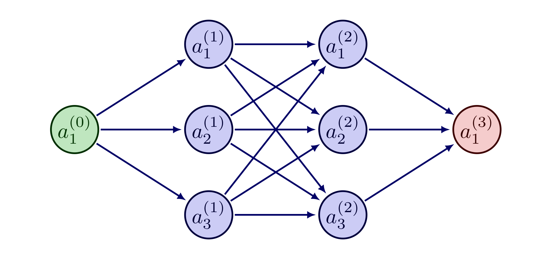
2. The NN_sinus model is created in with two hidden layers (hidden1 and hidden2) and ten neurons (def __init__(self):)
3. A slightly smaller (for visibility) model with two hidden layers and three neurons is presented below.
4. In the forward step, the nn.functional.relu(a_0) is used. It simply takes the input argument, $a_0=x_0$, multiplies it with a weight, $w$, adds a bias, $b$, and the ReLU actuator, $s$, is applied (see the activation functions below). The input, $a_1$, to the top neural in the first hidden layer is then $a_1 = s\{w_0 a_0 + b_0\}$. The expression in curly parenthesis is the argument in the ReLU activation function.

The forward step in the simplified model in the graph below is computed as follows.

First hidden layer.

\begin{eqnarray*} a_1^{(1)} &= s\left\{w_1^{(0)} a_1^{(0)} + b_1^{(0)} \right\} \\ a_2^{(1)} &= s\left\{ w_2^{(0)} a_2^{(0)} + b_2^{(0)} \right\} \\ & \vdots \\ a_{10}^{(1)} &= s\left\{ w_{10}^{(0)} a_{10}^{(0)} + b_{10}^{(0)} \right\} \end{eqnarray*}

Second hidden layer.

\begin{eqnarray*} a_1^{(2)} &= s\left\{w_1^{(1)} a_1^{(1)} + b_1^{(1)} + w_2^{(1)} a_2^{(1)} + b_2^{(1)} + w_3^{(1)} a_3^{(1)} + b_3^{(1)} \right\} \\ a_2^{(2)} &= s\left\{w_2^{(1)} a_1^{(1)} + b_1^{(1)} + w_2^{(1)} a_2^{(1)} + b_2^{(1)} + w_3^{(1)} a_3^{(1)} + b_3^{(1)} \right\} \\ & \vdots \\ a_{10}^{(2)} &= s\left\{w_{10}^{(1)} a_1^{(1)} + b_1^{(1)} + w_{10}^{(1)} a_2^{(1)} + b_2^{(1)} + w_{10}^{(1)} a_{10}^{(1)} + b_{10}^{(1)} \right\} \end{eqnarray*}

Output.

\begin{eqnarray*} a_3^{(3)} &= w_3^{(2)} a_1^{(2)} + b_1^{(2)} + w_3^{(2)} a_2^{(2)} + b_2^{(2)} \\ & \vdots \\ &+ w_{10}^{(2)} a_{10}^{(2)} + b_{10}^{(2)}\equiv Y \end{eqnarray*}

where $a_3^{(3)}$ is returned as the predicted $y$, i.e. $y_{pred}$.

Neural network. For visibility, I show only three neurons instead of ten. Two hidden layer which each have three neurons denoted by circles. The vectors between the neurons represent connections. Input: $a_1^{(0)}= x$; output: $a_1^{(3)} = y$

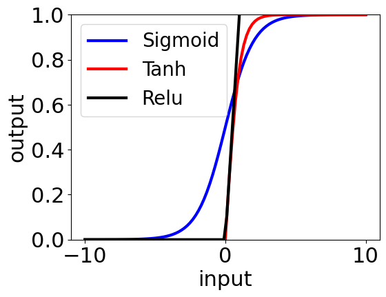
An activation function is the function which enables neural network to learn complex (non-linear) relationships by transforming the output of the previous layer. Without activation functions, neural network can only learn linear relationships. Three common activation functions are shown below.

Different activation functions. ReLU $=\max(0,x)$; Tanh $=\tanh(x)$; Sigmoid $=\left(1 + \exp(-x)\right)^{-1}$.

Predict a straight line using NN

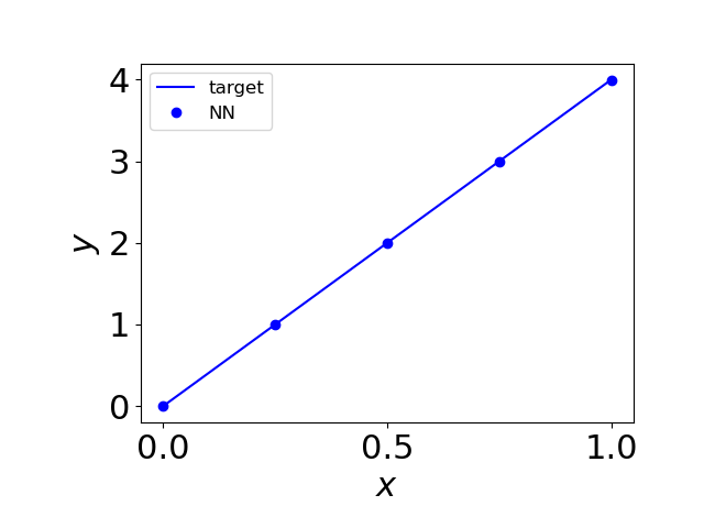
In order to better understand the forward step in NN, I will write a Python script without using PyTorch's activators and torch.nn.functional. I start be creating $x$ and $y$.

import torch
from torch import nn

x = torch.linspace(0, 1, 5)
y = 4*x

X = x.view(-1,1)
Y = y.view(-1,1)

Since I will predict a straight line, $y=x$, I don't need any activator. The NN model is built with the code below.

class NN_line(nn.Module):
    def __init__(self):
        super().__init__()
#axis 0: number of input
        self.input   = nn.Linear(1, 2)  
        self.hidden1 = nn.Linear(2, 2)
#axis 1: number of output
        self.hidden2= nn.Linear(2, 1)  
        self.input.bias.data.normal_(0.,1)
        self.input.weight.data.normal_(0.,1)
        self.hidden1.bias.data.normal_(0.,1)
        self.hidden1.weight.data.normal_(0.,1)
        self.hidden2.bias.data.normal_(0.,1)
        self.hidden2.weight.data.normal_(0.,1)
    def forward(self, x0):
        x1 = model.input.bias.view(-1,1) + \
            model.input.weight@x0.T
        x2 = model.hidden1.bias.view(-1,1) + \
              model.hidden1.weight@x1
        output_temp = model.hidden2.bias.view(-1,1) + \
              model.hidden2.weight@x2
        output = output_temp.view(-1,1)
        return output

Neural network for the straight line. Two hidden layer which each have two neurons denoted by circles.

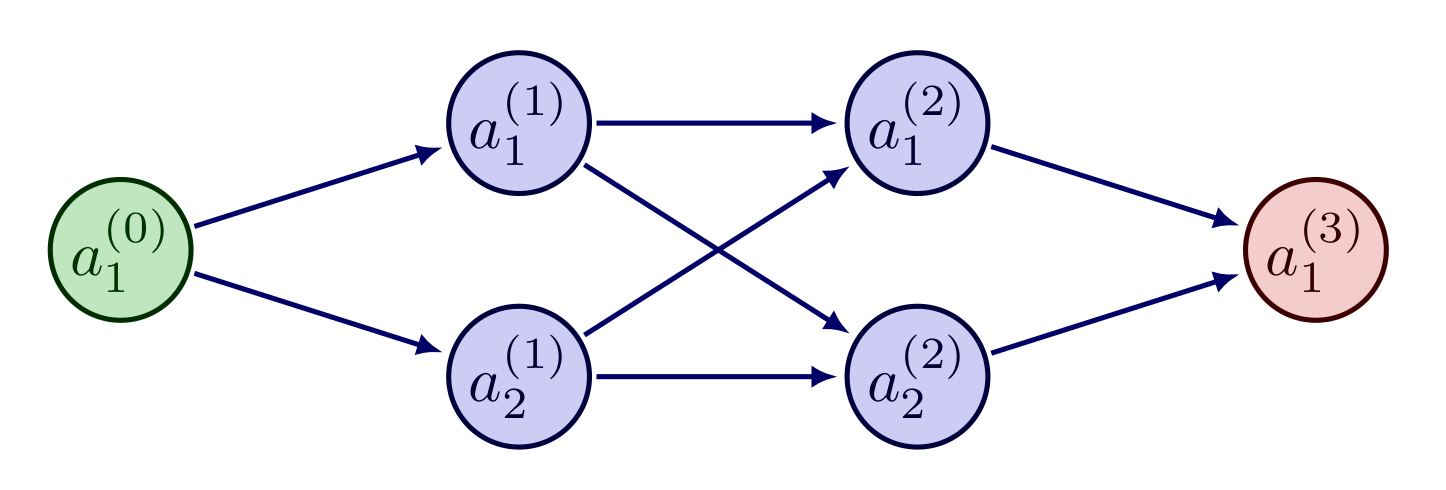
As can be seen in the figure above, I use two hidden layers and two neurons. All weights and biases are initialized as normal distribution with mean equal to zero and standard deviation equal to $1$. There is one input (axis 0 of input) and one output (axis 1 of hidden layer no 2).The forward step is coded as above.

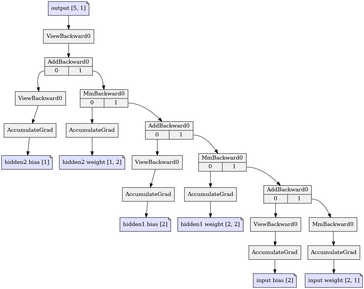
The commands .view(-1,1) and .T are used to reshape vectors between row and column vectors. The symbol '@' denotes matrix multiplication. The shapes of the weights biases are given below.

\begin{eqnarray*} \rm input.bias.view(-1,1)&=& \rm torch.Size([2, 5]) \\ \rm input.weight&=& \rm torch.Size([2, 1]) \\ \rm x0.T&=& \rm torch.Size([1, 5])\\ \rm output, x1&=& \rm torch.Size([2, 5]) \end{eqnarray*}

Above: input.bias.view(-1,1)[2,5] added to matrix multiplicaction of input.weight[2,1] and x0.T[1.5] which gives x1[2.5]. Note that the size of input.bias.view(-1,1) in the Python code really is [2,1] but Python takes care of this.

\begin{eqnarray*} \rm x1&=& \rm torch.Size([2, 5])\\ \rm hidden1.bias.view(-1,1)&=& \rm torch.Size([2, 5])\\ \rm hidden1.weight&=&\rm torch.Size([2, 2])\\ \rm output, x2&=&\rm torch.Size([2, 5]) \end{eqnarray*}

Above: hidden1.bias.view(-1,1)[2,5] added to matrix multiplicaction of hidden1.weight[2,2] and x1[2.5] which gives x1[2.5]. Regarding size of hidden1.bias.view(-1,1) in Python code, see comment above.

\begin{eqnarray*} \rm x2&=&\rm torch.Size([2, 5])\\ \rm hidden2.bias.view(-1,1)&=& \rm torch.Size([1, 5])\\ \rm hidden2.weight&=& \rm torch.Size([1, 2])\\ \rm output&=&\rm torch.Size([1, 5]) \end{eqnarray*}

Above: hidden2.bias.view(-1,1)[1,5] added to matrix multiplaction of hidden1.weight[1,2] and x2[2.5] which gives output[1.5]. Regarding size of hidden2.bias.view(-1,1) in Python code, see comment above.

Note that the weights and biases have the same values at all $x$ points.

The iteration loop to converge the NN model is given below (it is the same as above).

# Create the model
# the seed makes ensure that the same nomal distribution 
# is generated every time
torch.manual_seed(42)
model = NN_line()
# Define the loss function and the optimizer
loss_fn = nn.MSELoss()
# under-relaxation
alpha = 0.001   
optimizer = torch.optim.Adam(params = model.parameters(),\
                             lr = alpha)

max_iter = 1000
for n in range(max_iter):
    y_pred = model(X)
    loss = loss_fn(y_pred, Y)
    optimizer.zero_grad()
    loss.backward()
    optimizer.step()
    if n % 200 == 0:
      print(f'Iteration: {n}, loss: {round(loss.item(), 6)}')

Iteration: 0, loss: 1.936108
Iteration: 200, loss: 1.412122
Iteration: 400, loss: 0.795214
Iteration: 600, loss: 0.161624
Iteration: 800, loss: 0.003106

The figure below shows predicted $y = 4$

$y = 4x$

The autograd graph is seen below.

Autograd graph for $y=4x$

Cubic line

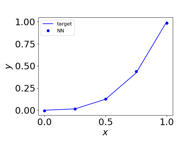
A final test case will be a cubic line. Since this is non-linear, I need to add an actuator. I choose the relu actuation function. I also need to use more neurons. The code for the straight line is modified as follows.

1. learning rate is set to $0.02$
2. $500$ epochs are used
3. I increase number of neurons from $2$ to $10$
4. In the forward step I multiply the two hidden layers with the relu actuator.

The Python code is given below.

import torch
import sys
import matplotlib.pyplot as plt
from torch import nn

plt.interactive(True)
plt.close('all')
plt.rcParams.update({'font.size': 22})

x = torch.linspace(0, 1, 5)
y = x**3

X = x.view(-1,1)
Y = y.view(-1,1)

# Build the model:
class NN_cubic(nn.Module):
    def __init__(self):
        super().__init__()
#axis 0: number of inputs
        self.input   = nn.Linear(1, 10) 
        self.hidden1 = nn.Linear(10, 10)
#axis 1: number of outputs
        self.hidden2= nn.Linear(10, 1)
        self.input.bias.data.normal_(0.,1)
        self.input.weight.data.normal_(0.,1)
        self.hidden1.bias.data.normal_(0.,1)
        self.hidden1.weight.data.normal_(0.,1)
        self.hidden2.bias.data.normal_(0.,1)
        self.hidden2.weight.data.normal_(0.,1)

    def forward(self, x0):
        x1 = model.input.bias.view(-1,1) \
         +  model.input.weight@x0.T
        x1 = torch.maximum(x1,torch.tensor(0.))  # ReLU

        x2 = model.hidden1.bias.view(-1,1) \
           + model.hidden1.weight@x1
        x2 = torch.maximum(x2,torch.tensor(0.))  # ReLU

        output_temp = model.hidden2.bias.view(-1,1) \
                    + model.hidden2.weight@x2
        output = output_temp.view(-1,1)

        return output

# Create the model
# the seed makes ensure that the same nomal 
# distribution is generated every time
torch.manual_seed(42)
model = NN_cubic()

# Define the loss function and the optimizer
loss_fn = nn.MSELoss()
# learning_rate = 0.0001
learning_rate = 0.02 #reduce the learning rate for stability
print(' model.parameters()', model.parameters())
print(' model', model)
optimizer = torch.optim.Adam(params = model.parameters(),
                            lr = learning_rate)

# Train the model
epochs = 500
epoch_num = []
train_losses = []
test_losses = []
for epoch in range(epochs):
    y_pred = model(X)
    loss = loss_fn(y_pred, Y)
    optimizer.zero_grad()
    loss.backward()
    optimizer.step()
    if epoch % 100 == 0:
      print(f'Epoch: {epoch}, loss: {round(loss.item(), 6)}')

 model.parameters() <generator object Module.parameters at 0x7f9c16405fc0>
 model NN_cubic(
  (input): Linear(in_features=1, out_features=10, bias=True)
  (hidden1): Linear(in_features=10, out_features=10, bias=True)
  (hidden2): Linear(in_features=10, out_features=1, bias=True)
)
Epoch: 0, loss: 15.925939
Epoch: 100, loss: 0.009603
Epoch: 200, loss: 0.004847
Epoch: 300, loss: 0.00246
Epoch: 400, loss: 0.000738

The predicted line is shown in the figure below.

$y = x^3$

References

• Francois Fleuret, "The Little Book of Deep Learning"
• Tensors and Gradients in PyTorch
• What PyTorch Really Means by a Leaf Tensor and Its Grad
• A Gentle Introduction to torch.autograd
• Partial Derivatives Chain Rule using torch.autograd.grad
• Understanding pytorch’s autograd with grad_fn and next_functions
• Understanding the ErrorL A leaf Variable that requires grad is being used in an in-place operation
• The Fundamentals of Autograd
• How to Visualize PyTorch Neural Networks - 3 Examples in Python
• Automatic Differentiation with torch.autograd
• PyTorch for Automatic Gradient Descent
• 3Blue1Brown: But what is a neural network
• 3Blue1Brown: gradient descent, how neural networks learn
• 3Blue1Brown: backpropagation, intuitively
• 3Blue1Brown: backpropagation, calculus
• Sebastian Lague: how to create a neural network
• PyTorch Autograd Explained - In-depth Tutorial